An Introduction to Linear Programming
Purplemath
What is linear programming?
Linear programming is the process of taking various linear inequalities (called "constraints") relating to some situation, and finding the best value obtainable under those conditions. A typical example would be taking the limitations of materials and labor, and then determining the optimal production levels for maximal profits under those conditions.
Content Continues Below
Is linear programming useful in real life?
Affiliate
Advertisement
In real life, linear programming is part of a very important area of mathematics called "optimization techniques".
This field of study (or at least the applied results of it) are used every day in the organization and allocation of resources. These real life systems can have dozens of variables, or hundreds, or more. (For the curious, a history of linear programming: PDF)
In algebra, though, you'll only work with the simple (and graphable) two-variable linear case.
How do you solve a linear programming problem?
Affiliate
The general process for solving linear-programming exercises is as follows:
- Graph the system of linear inequalities. The area walled off by the various inequalities is called the "feasibility region".
- Taking the "equals" versions of the inequalities, solve pairs of lines to find the corner points (or "vertices") of the feasibility region.
- Plug the coordinates of each of the vertices into the model for the situation at hand (that is, into the optimization equation).
- If you're maximizing, take the corner that gives you the highest value; otherwise, take the one with the lowest value.
- For word problems, interpret the result within the context given (for example, say "eight meters wide and three meters tall" rather than just "(8, 3)").
Why do you test only the corners?
Somebody figured out that, given a system of linear inequalities and an equation to be optimized (that is, to be maximized or minimized), the system's optimal solution will always be on a corner.
There are complicated explanations for this, but also intuitive ones (for the simple two-variable case that we'll be working with). Either way, the corners are where it's at.
Content Continues Below
- Find the maximal and minimal value of z = 3x + 4y subject to the following constraints:
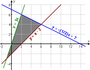
The three inequalities in the curly braces are the constraints. The area of the plane that they mark off will be the feasibility region. The formula "z = 3x + 4y" is the optimization equation. I need to find the (x, y) corner points of the feasibility region that return the largest and smallest values of z.
My first step is to solve each inequality for the more-easily graphed equivalent forms:
It's easy to graph the system; you take the "equals" version of each inequality (these "equals" versions being the lines forming the edges of the feasibility region), and solve the system of linear equations formed by each pair of lines:

To find the corner points — which aren't always clear from the graph — I'll pair the lines (thus forming a system of linear equations) and solve:
y = 3x
−x + 14 = 6x
14 = 7x
2 = x
y = 3(2) = 6
corner point at (2, 6)
y = x − 2
−x + 14 = 2x − 4
18 = 3x
6 = x
y = (6) − 2 = 4
corner point at (6, 4)
y = 3x
y = x − 2
3x = x − 2
2x = −2
x = −1
y = 3(−1) = −3
corner point at (−1, −3)
So the corner points — the points I'll be plugging into the optimization equation — are (2, 6), (6, 4), and (−1, −3). To find the solution to this exercise, I only need to plug these three points into "z = 3x + 4y".
(2, 6): z = 3(2) + 4(6) = 6 + 24 = 30
(6, 4): z = 3(6) + 4(4) = 18 + 16 = 34
(−1, −3): z = 3(−1) + 4(−3) = −3 −12 = −15
Then the maximum of z = 34 occurs at (6, 4),
and the minimum of z = −15 occurs at (−1, −3).
As you can see, solving a linear-programming exercise can be a lengthly process, but each individual step is fairly straightforward. Just take your time, label clearly, and work neatly, and you'll get it!
URL: https://www.purplemath.com/modules/linprog.htm
Select a Course Below
Standardized Test Prep
Homeschool Math
© 2024 Purplemath, Inc. All right reserved. Web Design by ![]()


