Systems of Linear Inequalities: Solving by Graphing
Purplemath
Once you've learned how to graph two-variable linear inequalities, you can move on to solving systems of two-variable linear inequalities.
What is a system of linear inequalities?
A "system" of two-variable linear inequalities is a set of linear inequalities for which each of the inequalities is drawn on the same graph. On this graph, you shade the side of each line that is included in that line's inequality.
Content Continues Below
What is the solution to a system of linear inequalities?
The solution to the system of linear inequalities is the region of the plane where all of the individual lines' shading overlaps. This solution region is the intersection of the various lines' shadings; it is the area of the graph where all the inequalities are "happy".
What is an example of solving a system of linear inequalities?
- Solve the following system:
2x − 3y ≤ 12
x + 5y ≤ 20
x > 0
Just as with solving single linear inequalities, it is usually best to solve as many of the inequalities as possible for "y" on one side. Solving the first two inequalities, I get the rearranged system:
Advertisement
y ≥ (2/3) x − 4
y ≤ (−1/5) x + 4
x > 0
Affiliate
"Solving" systems of two-variable linear inequalities means "graphing each individual inequality, and then finding the overlaps of the various solutions". So I graph each inequality individually, marking the "solution" side of each line as I go, and then I'll find the overlapping portion of the various solution regions.
The line for the first inequality in the above system, y ≥ (2/3) x − 4, looks like this:
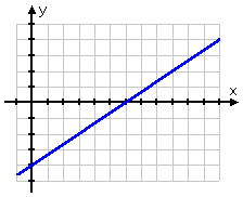
The above line, shown in blue, represents the line y = (2/3) x − 4. The inequality part will be indicated by shading one side or the other of this line.
This inequality is an "or equal to" inequality, so the line is drawn as a solid line, rather than as a dashed line.
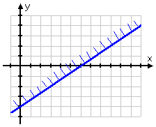
This inequality is a "greater than" inequality, so I want to shade above the line. However, since there will be more than one inequality on this graph, I don't know (yet) how much of that upper side of this line I will actually need.
Content Continues Below
How do I keep track of where the end solution region will be?
Until I know how much of a given single inequality's solution region I'll need, I can keep track of the fact that I want a certain side of an inequality's line (in this case, the top region) by drawing a little "fringe" along the top side of my solid line, like this:
Now I'll graph the line for the second inequality they gave me; namely, y ≤ (−1/5) x + 4:
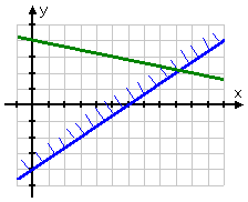
This is another "or equal to" inequality, so the line is solid; and, since this is a "less than" inequality, I'll draw the fringe along the bottom of my solid line:
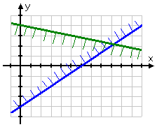
Affiliate
The last inequality is a common "real life" constraint, restricting the variable x to being positive only. The line "x = 0" is just the y-axis, and I'll be wanting to shade the right-hand side. Because this is a strict inequality (that is, this inequality is not an "or equal to" inequality); the boundary (namely, the line dashed along the y-axis) is not to be included in the solution to the system:
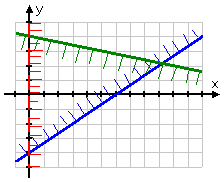
The "solution" of the system is the region where all the inequalities are happy; that is, the solution is where all the inequalities work, the region where all three individual solution regions overlap. In this case, the solution is the shaded part in the middle:
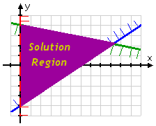
The answer to this sort of exercise is typically a graph, as shown above. Nothing further should be required.
Notice how, in my graph, I made sure that the dashed line for the "x > 0 inequality is still clearly visible as being a dashed line. When your answer is a picture like this, make sure to draw it clearly. You're welcome to shade in your solution region right up to (and maybe onto) the solid lines, but make sure that your dashed lines are clearly dashed — by heavily over-drawing them, or maybe using a different color for contrast, if necessary. But make your meaning clear!
The solution region for the system graphed above is called a "bounded" solution, because there are lines closing it in on all sides. That is, the solution region is a bounded (finite) geometric figure; in the case above, the solution region was a triangle.
URL: https://www.purplemath.com/modules/syslneq.htm
Select a Course Below
Standardized Test Prep
Homeschool Math
© 2024 Purplemath, Inc. All right reserved. Web Design by ![]()


