A Four-Variable Word Problem
Purplemath
In the previous exercise, there were three inputs that I had to consider, but I had only two variables. The way I dealt with that was to assign meaning to the two usual variables, x and y; then I created an expression for the third input by subtracting the first two variable expressions from the given total.
Content Continues Below
But what if there are more inputs than just three?
(Full disclosure: It took me a while to figure out how to approach the exercise below. Don't feel like you're "stupid" or something, just because it takes you some time to get started on harder exercises. They *are* harder, so they *should* take more time. Work hard, but be less hard on yourself!)
- A building supply has two locations in town. The office receives orders from two customers, each requiring 3/4-inch plywood. Customer A needs fifty sheets and Customer B needs seventy sheets.
The warehouse on the east side of town has eighty sheets in stock; the west-side warehouse has forty-five sheets in stock. Delivery costs per sheet are as follows: $0.50 from the eastern warehouse to Customer A, $0.60 from the eastern warehouse to Customer B, $0.40 from the western warehouse to Customer A, and $0.55 from the western warehouse to Customer B.
Find the shipping arrangement which minimizes costs.
Hmm... I've got four things to consider, being the four possible paths (the "shippng arrangement") of the plywood sheets:
- from east warehouse to Customer A
- from east warehouse to Customer B
- from west warehouse to Customer A
- from west warehouse to Customer B
Affiliate
But I only have two variables. How can I handle this?
The variables obviously need to stand for the number of sheets being shipped, but I have four different sets of sheets. This calls for subscripts and explicit labelling:
- shipped from east warehouse to Customer A: Ae
- shipped from west warehouse to Customer A: Aw
- shipped from east warehouse to Customer B: Be
- shipped from west warehouse to Customer B: Bw
Since Customer A wants 50 sheets and Customer B wants 70 sheets, then:
Ae + Aw = 50, so Aw = 50 − Ae (Equation I)
Be + Bw = 70, so Bw = 70 − Be (Equation II)
Since the eastern warehouse can ship no more than eighty sheets and the western warehouse can ship no more than forty-five sheets, then:
0 ≤ Ae + Be ≤ 80
0 ≤ Aw + Bw ≤ 45
And the optimization equation will be the shipping cost, since they'll want to minimize the cost of getting their product to their customers:
C = 0.5Ae + 0.6Be + 0.4Aw + 0.55Bw
Content Continues Below
Where does this leave me? The equations (labelled as Equations I and II above) allow me to substitute and get rid of two of the variables in the second inequality above, so:
0 ≤ Ae + Be ≤ 80
0 ≤ (50 − Ae) + (70 − Be) ≤ 45
Simplifying the second inequality above gives me the new system:
0 ≤ Ae + Be ≤ 80
0 ≤ 120 − Ae − Be ≤ 45
Advertisement
Multiplying through by −1 (thereby flipping the inequality signs) and adding 120 to all three "sides" of the second inequality, I get the new system:
0 ≤ Ae + Be ≤ 80
120 ≥ Ae + Be ≥ 75
I'm more comfortable with my inequalities in this context being less-than's, so I'll flip that second inequality around:
0 ≤ Ae + Be ≤ 80
75 ≤ Ae + Be ≤ 120
I know that Ae + Be has to be no less than (that is, must be more than) 75 and no more than (that is, must be less than) 80. Then these two inequalities reduce to one:
75 ≤ Ae + Be ≤ 80
I can also use Equations I and II to simplify the optimization equation:
C = 0.5Ae + 0.6Be + 0.4Aw + 0.55Bw
= 0.5Ae + 0.6Be + 0.4(50 − Ae) + 0.55(70 − Be)
= 0.1Ae + 0.05Be + 58.50
Affiliate
Due to the size of the orders, I have:
0 ≤ Ae ≤ 50
0 ≤ Be ≤ 70
Since I have only two variables now, and since I'll be graphing with x and y, I'll rename the two remaining variables:
x = Ae
y = Be
Then my entire system is as follows:
Minimize C = 0.1x + 0.05y + 58.50, subject to the following:
x ≥ 0
y ≥ 0
y ≥ −x + 75
x ≤ 50
y ≤ 70
y ≤ −x + 80
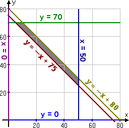
The feasibility region graphs as:

The corner points are (5, 70), (10, 70), (50, 30), and (50, 25). When you test these points in the optimization equation, you should get the minimum cost when you ship as follows:
5 sheets from the eastern warehouse to Customer A
70 sheets from the eastern warehouse to Customer B
45 sheets from the western warehouse to Customer A
0 sheets from the western warehouse to Customer B
URL: https://www.purplemath.com/modules/linprog5.htm
Select a Course Below
Standardized Test Prep
Homeschool Math
© 2024 Purplemath, Inc. All right reserved. Web Design by ![]()


